Algorithms for Beginners: Data Pruning With Boundaries

What is Pruning

In algorithms, sometimes you will have to do calculations on massive data sets, concerning yourself with either 3D grids of billions or trillions of cells, or possibly have to map ranges of similar sizes. Often times, if you simply try to do the calculations directly or naively, you will spend days to compute a desired answer or use gigabytes of memory when often times you can get a result in fractions of a second with less the a kilobytes of memory. The key strategy is pruning. What pruning is instead of calculating every possible answer, you instead start by using your knowledge of the set of data to either completely eliminate a large amount of data that you know can’t possibly be the answer, or group large amounts of data and represent that as a single block, because you know every element of this block will always have the same state.

A perfect example of how to use pruning is Advent of Code 2023 Day 5, which has us try to map ranges of seeds to locations, with those ranges being billions of elements long, and here is how it is done.

The Problem

Advent of Code 2023 Day 5 asks us to translate a set of seeds to their appropriate soil, then translate that to its appropriate fertilizer, then water, light, temperature, humidity, and finally location. With the idea of finding the minimum location among all the initial seeds.

Explaining The Input Data

The full sample input data looks like this.

seeds: 79 14 55 13

seed-to-soil map:
50 98 2
52 50 48

soil-to-fertilizer map:
0 15 37
37 52 2
39 0 15

fertilizer-to-water map:
49 53 8
0 11 42
42 0 7
57 7 4

water-to-light map:
88 18 7
18 25 70

light-to-temperature map:
45 77 23
81 45 19
68 64 13

temperature-to-humidity map:
0 69 1
1 0 69

humidity-to-location map:
60 56 37
56 93 4

For each row within a particular map, the numbers in order represent:

1. the start of the output range
2. the start of the input range
3. the size of the mapping range

So a row \(\text{X Y Z}\) maps an input range \([Y, Y+Z) \to [X, X+Z)\) in a one to one fashion. So for the light-to-temperature map’s 45 77 23, light will be mapped to temperature like

\[77 \to 45\] \[78 \to 46\] \[79 \to 47\] \[...\] \[100 \to 68\]

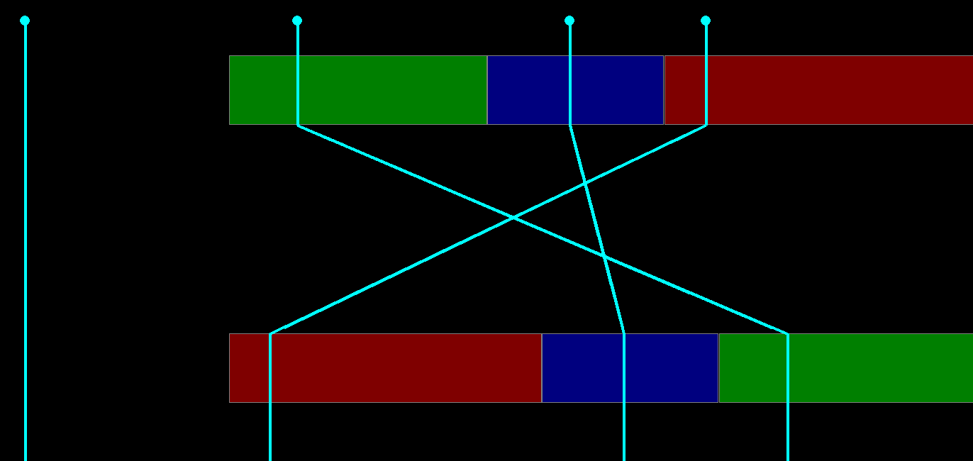
Now these only represent one possible maps. However light-to-temperature has three mappings, so when translating lights to temperature, we have to check which among all 3 ranges is mapped, and apply that mapping. There are no mapping, you just map to the same value.

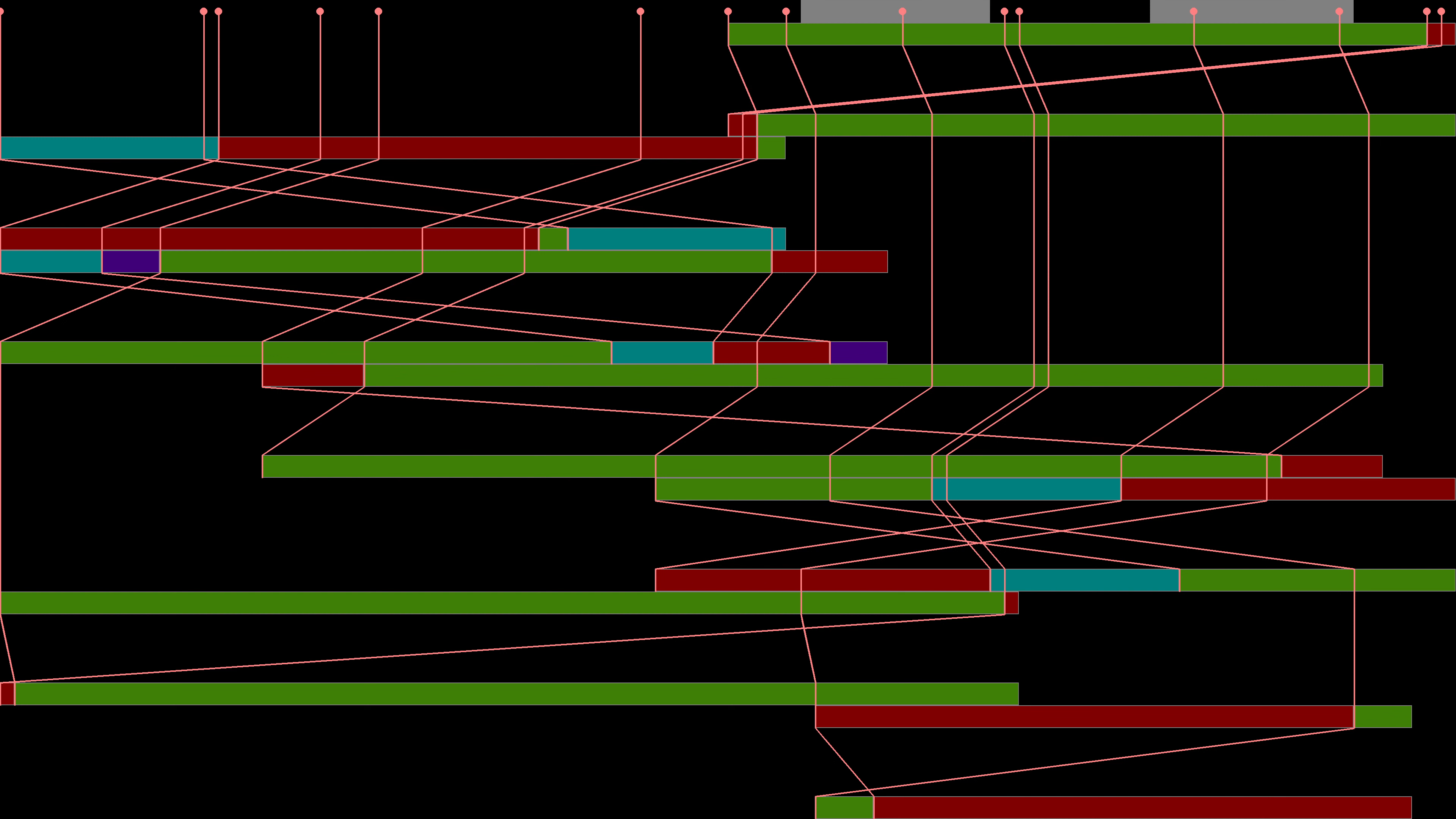
Personally, I like to imagine these as multiple layers of squares with invisible parallelograms guiding paths from the source to the destination among parallel lines.

The actual puzzle involves mapping each of the starting seeds to their corresponding location to find the smallest location. A rather simple task, something that anyone who passes Programming 101 could code. But this is not the interesting part. The interesting part comes up in part 2, when you start having to deal with impossibly large number of seeds to deal with?

Part 2: TEN BILLION SEEDS

Large Data Set

After solving part 1, part 2 redefine what the seeds line means in the input file. Instead of each number being a seed, each pair of number represent a range of seeds, where the first number is the start of the range, and the second number is the length of the range. So in the example, 79 14 55 13 represent the seed ranges \([79, 93)\) and \([55, 68)\). Now increasing from 4 seeds to 27 seeds isn’t that much, you can just run the data through the same algorithm as part 1 and get an answer quickly, however there is one major snag: this is just the test data.

Now the actual input data is different per person, but my input data is uh… kinda large. In my case, the total number of seeds I have to consider is 1 421 233 717, which needless to say might take a while to compute the same way as part 1.

seeds: 2019933646 2719986 2982244904 337763798 445440 255553492 1676917594 196488200 3863266382 36104375 1385433279 178385087 2169075746 171590090 572674563 5944769 835041333 194256900 664827176 42427020

Pruning Ranges

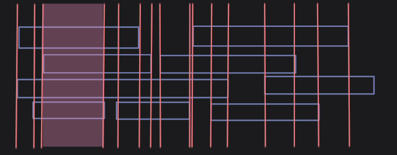
When dealing with large ranges, it can often been beneficial to instead of thinking of every discreet value, but instead consider the boundaries of those values.

You can see in the more ⭐ 𝓐𝓫𝓼𝓽𝓻𝓪𝓬𝓽 ⭐ representation of a problem involving a set of ranges, we can look solely at the boundaries, because everything between boundaries (like the shaded region), all pretty much do the same things.

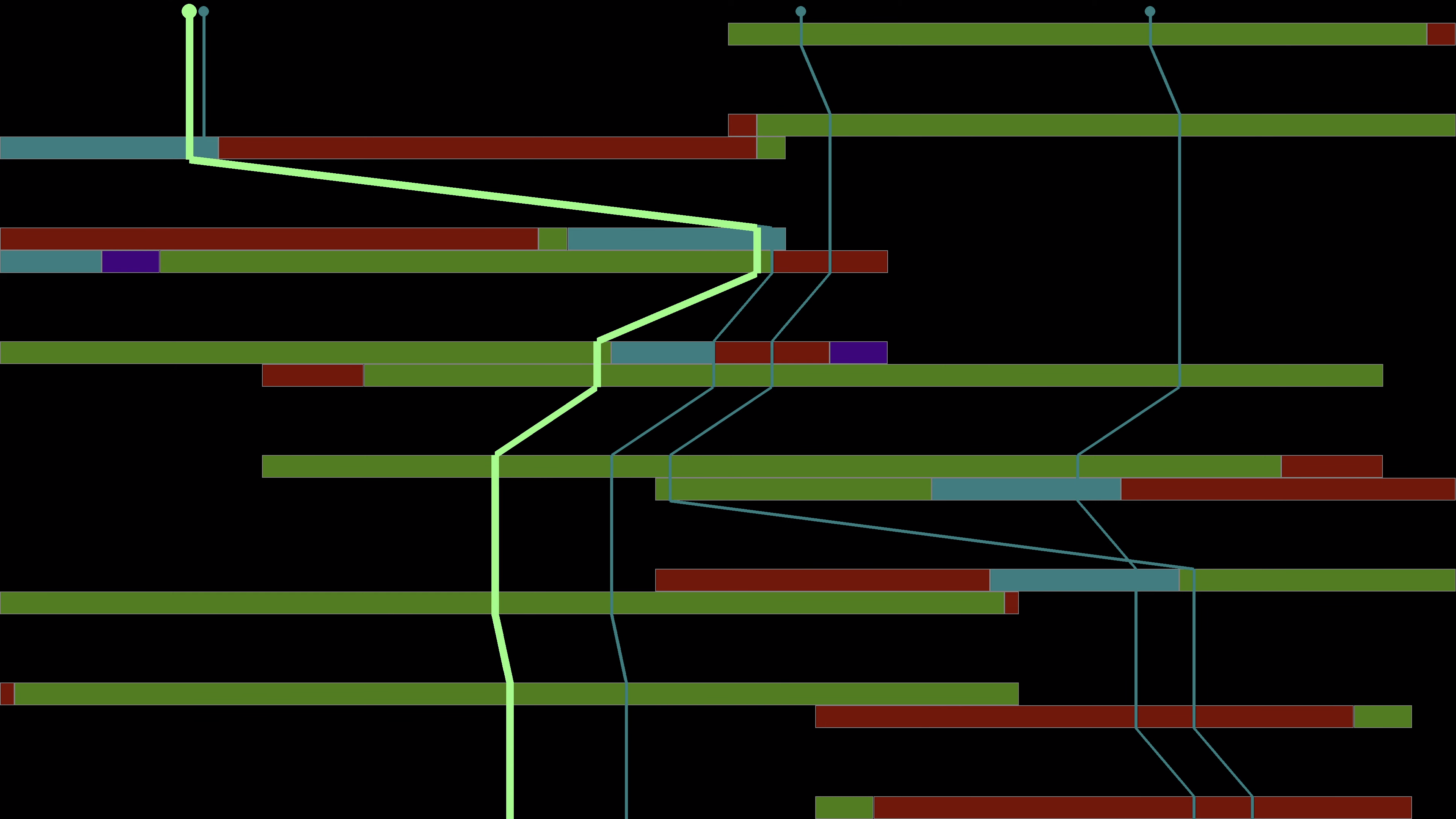
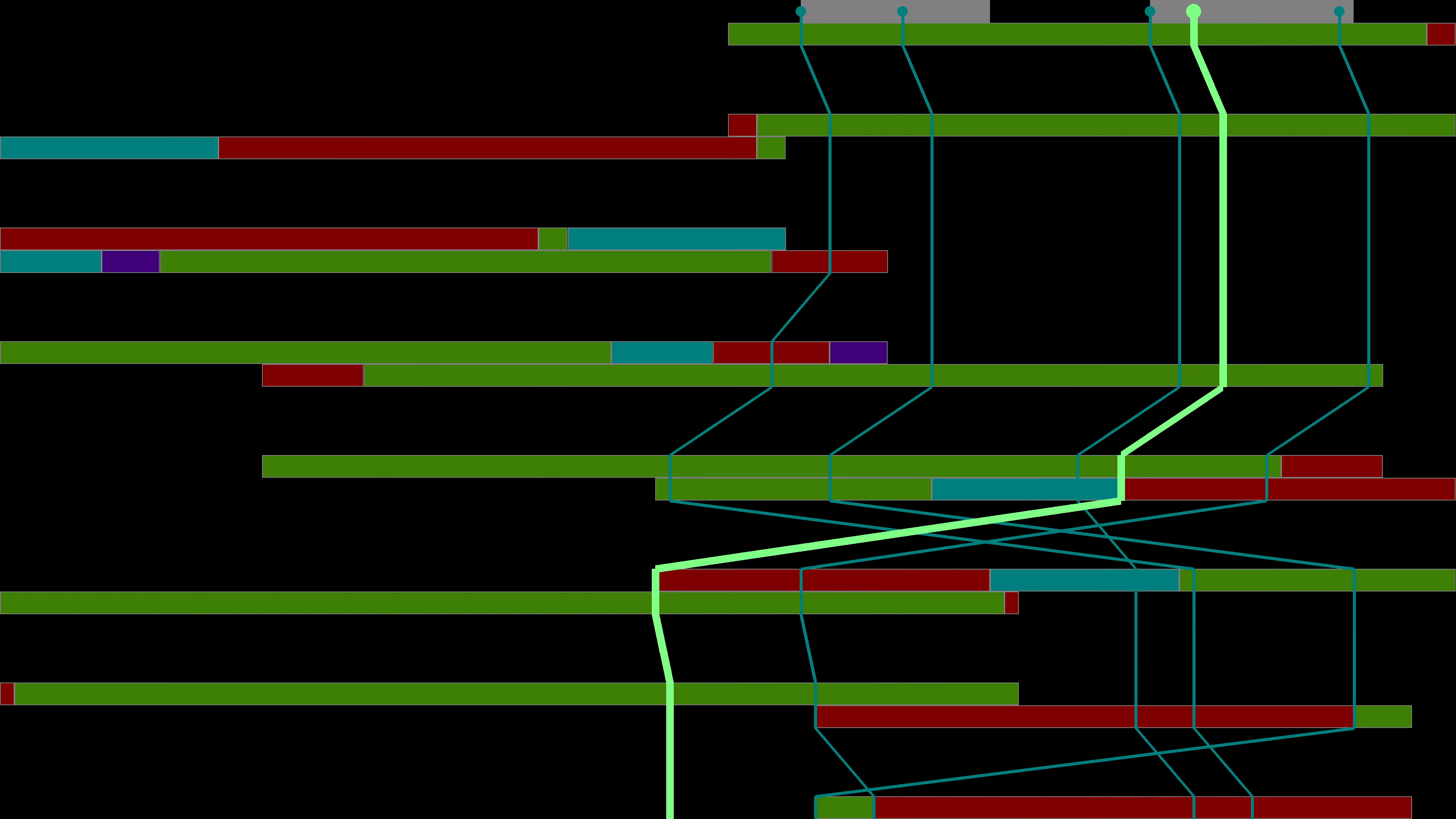
In the more Concrete example of our seed map, using the sample data again, we can see something like this play out. Everything between the two green lines go through all of the same maps. Even one seed to the right of the boundary would split off from the range and follow the red box of the 4th map.

This has a particular interesting property. Since we are specifically looking for the seed with the smallest location after mapping, we know for a fact that within any given boundary range, it is the leftmost seed that produced the smallest location, simply because \(f(x+n) = f(x) + n\) if \(x+n\) and \(x\) are both in the same boundary set. So that begs the question, how do we find these boundaries? Well by working backwards of course.

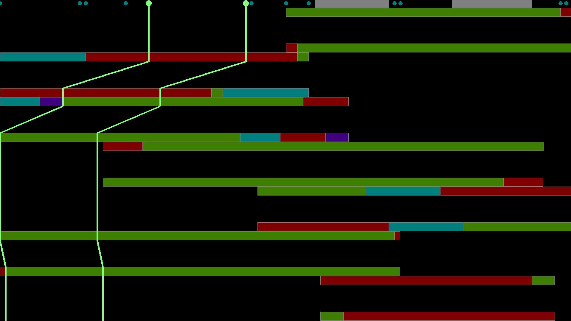
What we ultimately have to do is for any boundary in any level, we have to reverse the map to find out which seeds pass through that boundary. To do this we can start at the locations level, take all of its left boundaries, then reverse the seed → location map, to get a location → seed map. Then we take all of the humidity boundaries, apply the humidity → seed map, etc.

After all that work, we should have a list of every seed whose map touches the leftmost boundary of one of the layers of the map. Of course we then have to narrow down these seeds to though actually in one of the starting ranges we get. Also when filtering, don’t forget to add the left boundary of the seeds as well, just in case the boundary set represented by the first seed to the left of the seed range results in the minimum location.

This process narrowed down the list of possible seeds to consider from over a billion to just around 50, saving a lot of time and space. Now we just run this new set of seeds through the same process as Part 1, and we will get our answer

Animation

To see the fully animation of these algorithms in action, check out these youtube videos. First is the algorithm working on the sample data, and the second is the algorithms working on my actual input data.